
Graph Based Recommender Systems
In this post I present the theory for the topic of my MSc thesis titled “Graph based Recommender Systems for Implicit Feedback” - we’ll go through and motivate in detail our new model called Implicit Graph Convolutional Matrix Completion (iGC-MC), an extension of a once state-of-the-art method for explicit ratings prediction called GC-MC. If you’re new to recommender systems, check out my brief introduction before diving in.
Introduction
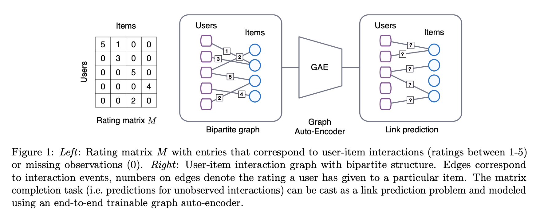
Broadly speaking the role of a recommender system is to fill in the missing entries of our sparse observation matrix $R$, where each entry $r_{ui}$ represents an interaction between a user and item. Graph Convoluation Matrix Completion (GC-MC) views this problem of matrix completion on our observation matrix $R$ from the point of view of link prediction on graphs. In GC-MC, the interaction data is represented using bipartite user-item graph with labeled edges denoting observed ratings or interactions. Building on recent progress in deep learning on graph-structured data, the method proposes a graph auto-encoder framework based on differentiable message passing on the bipartite interaction graph. GC-MC when published achieved state-of-the-art performance on the famed MovieLens dataset, which formed a large part of my motivation in adapting the method for implicit feedback whilst also persuing an interest in Graph Neural Networks (introduced below).
Graph Neural Networks
GNNs are one of the hot topics in ML at the moment and rightly so - several studies on extending deep learning methods for graph data have emerged in recent years (link to survey paper). Data generated from non-Euclidean domains, represented by graphs that capture complex relationships and interdependency between objects, had previously imposed significant challenges on existing machine learning algorithms. But these powerful new approaches allow learning to be performed with a vast range of potential applications in domains ranging from drug discovery to e-commerce. A key step was in the development of Graph Neural Networks (GNNs) was to generalise the operation of convolution from grid data to graph data. The core idea of a Graph Convolutional Network (GCN) is to generate the representation of a node by aggregating its own feature with its neighbours’ features, a form of message passing. Subsequent layers then build information about the 2nd and 3rd order neighbourhoods of the node, thereby building a powerful representation of the graph (great post on GCNs, also in Further Reading). Graph autoencoders (GAEs) are deep neural architectures that map nodes into latent feature space then decode relevant graph information from latent representations.
Implicit Feedback
Why is a recommender system trained to predict ratings different to one that predicts clicks? Well, the numerical value of explicit feedback represents preference (a star rating 1-5), whilst in the implicit setting feedback (e.g. clicks, purchases, views, playcounts) indicates confidence. We formalise this notion by defining the following matrix of binary variables $P = (p_{ui}){N\times M}$ where $p{ui}=0$ if $r_{ui} = 0$ or $p_{ui}=1$ when $r_{ui} \neq 0$.
That is, $p_{ui}$ represents whether user $u$ has interacted with item $i$ at all. Due to the inherently noisy nature of implicit data, our belief in each value $p_{ui}$ has varying levels of confidence associated with them. We introduce the set of variables $c_{ui}$ that measure our confidence in observing $p_{ui}$. We consider two plausible choices for $c_{ui}$, both monotonic increasing transformations of our observations $r_{ui}$:
\[\begin{aligned} {c}_{ui} &= 1 + \alpha {r}_{ui} \\ {c}_{ui} &= 1 + \alpha \log(1 + {r}_{ui}/\epsilon) \end{aligned}\]The benefit of these transformations is also to better model data with a heavy skew. These serve the purpose of giving some minimal unit confidence for every $p_{ui}$, whilst giving an increasing confidence for larger observations. The parameter $\alpha$ controls this rate of increase: larger values of $\alpha$ places more weight on the observed entries whilst decreasing the parameter places more weight on the zero entries. The parameter $\epsilon$ in the logarithmic transform allows us to scale larger values down, which proves helpful in removing a power user bias, in which a small set of users carry a significant weight.
Constructing iGC-MC
Preliminaries
Consider the observation matrix $R$ of size $N \times M$ which we split into the matrix of binary values $P$ and its corresponding confidence matrix $C$, where we have applied an appropriate logarithmic or linear transformation as described above. We can represent this information as an undirected graph $G = (\mathcal{W},\mathcal{E})$ with entries as user nodes $n_u \in \mathcal{U}$ with $u\in{1,…,N}$ and item nodes $n_i \in \mathcal{V}$ with $i\in{1,…,M}$, such that $\mathcal{U}\cup \mathcal{V}=\mathcal{W}$. The edges $(n_u,c_{ui},n_i) \in \mathcal{E}$ have weights corresponding exactly to the confidence $c_{ui} \in \mathbb{R}^{\geq0}$ of our observation $p_{ui}\in {0,1}$, interpreted as a positive `count’ of how many times user $u$ has interacted with item $i$. Of importance is that unobserved user-item pairs ($r_{ui}=0$) are absent in this graph but do indeed factor into the method at a later stage. Note that the adjacency matrix of this graph $A$ is exactly our original observed ratings matrix $R$, we use these terms interchangeably going forward.
In the original formulation of GC-MC for explicit feedback, the undirected graph $G=(\mathcal{W},\mathcal{E},\mathcal{R})$ had a third attribute $\mathcal{R}={1,…,r_{max}}$. These were the labels of each edge, which represented the ordinal rating levels such as movie ratings from ${1,…,5}$. For the implicit feedback setting we have one single ordinal category: $\mathcal{R}=1$, indicating whether or not that edge represents an interaction between user $u$ and item $i$.
Graph auto-encoders in general comprise of an encoder $Z = f(O,A)$ that has as input a feature matrix $O$ of size $n \times d$, with $n$ the number of nodes and $d$ number of features, as well as an adjacency matrix $A$ to produce a node embedding matrix $Z=[z_1^T,…,z_N^T]^T$ of size $n \times f$, where $f$ is the latent dimension size. This is followed by a pairwise decoder model $\hat{A}=g(Z)$ which takes a pair of node embeddings $(z_i,z_j)$ and predicts respective entries in the new adjacency matrix $\hat{A}$.
For a bipartite implicit recommender system $G = (\mathcal{W},\mathcal{E})$ we reformulate the above as follows. The encoder is $[X,Y]=f(O,A)$ where $A \in \mathbb{R}^{N\times M}$ is the now the weighted adjacency matrix, with entries corresponding to confidence levels. The matrices $X$ and $Y$ correspond to user and item embeddings and are of shape $N \times f$ and $M \times f$, with $f$ the embedding size. Decoder: $\hat{A}=g(X,Y)$, a function acting on the user and item embeddings and returning a reconstructed rating matrix $\hat{A}$ of shape $N\times M$.
 GC-MC model structure for explicit feedback. From original paper
Graph convolution encoder
The encoder of our model uses a graph convolutional layer to perform local operations that gather information from the first-order neighbourhood of a node. These are a form of message-passing, where messages that are vector-valued are passed and transformed across edges of the graph. First the message from each node is formed, where a transformation is applied to the initial node vectors, which is the same across all locations (nodes) in the graph. Each message $\mu_{a \to b} \in \mathbb{R}^h$ has dimension $h$, a hyperparameter of the model. Messages take the following form, here from item node $i$ to user node $u$:
\[\begin{aligned} \mu_{i \to u} = Wo_i \end{aligned}\]where $W \in \mathbb{R}^{h \times d}$ is a parameter matrix that is to be learned during training, which maps the initial feature vector $o_i \in \mathbb{R}^d$ into $\mu_{i \to u} \in \mathbb{R}^h$. Messages from users to items $\mu_{u \to i}$ are calculated in an analogous way.
After the message-passing step, we sum the incoming messages to each node, multiplying each message by weight $\bar{c}_{ui}$ to result in a single intermediate vector denoted $h_i$, that represents a weighted average of messages. This is referred to as the graph convolutional layer:
\[\begin{aligned} h_u = \sigma \big( \sum_{i \in \mathcal{N}_u} \bar{c}_{ui} \mu_{i \to u} \big) \end{aligned}\]Here the sum is taken over the neighbours of node $n_{u}$ and $\sigma(\cdot)$ denotes an element-wise non-linear activation function chosen to be $ReLU(\cdot)=\max(0,\cdot)$. We normalise each message with respect to the in-degree of each node where each message is weighed by the edge label (i.e. the confidence parameter $c_{ui}$ associated with the observation between user $u$ and $i$):
\[\begin{aligned} \bar{c}_{ui} = \frac{c_{ui}}{\sum_{i \in \mathcal{N}_u} c_{ui}} \end{aligned}\]The motivation for use of such a weighting is so that the messaging passing step forms a weighted average of all incoming messages to that node. To arrive at the final embedding of user node $u$ we passs the intermediate output $h_u$ through a fully-connected dense layer:
\[\begin{aligned} x_u = \sigma(W'h_u) \end{aligned}\]where $W’ \in \mathbb{R}^{f \times h}$ is a separate parameter matrix to be learnt during training. The item embedding $y_i$ is calculated analogously with the same parameter matrix $W’$ or if side-information is included we use separate parameter matrices for user and item nodes.
We mention here, as in the original GC-MC paper that instead of a simple linear message transformation, variations are possible such as $\mu_{i \to u}=nn(o_u,o_i)$ where $nn$ is a neural network itself. In addition, instead of choosing a specific normalisation constant for individual messages, one could deploy some a form of attention mechanism, explored in some recent work.
Bilinear decoder
To reconstruct links in the bipartite interaction graph the decoder produces a probability of user $u$ and item $i$ interacting as follows:
\[\begin{aligned} \hat{a}_{ui} = p(A_{ui} > 0) = \sigma(x_u^T Q y_i) \end{aligned}\]where $Q$ is a trainable parameter matrix of shape $f \times f$. Here $\sigma(x)=1/(1+e^{-x})$ is the usual sigmoid function that maps the bilinear form into $[0,1]$ so that we gain a probabilistic interpretation of our output.
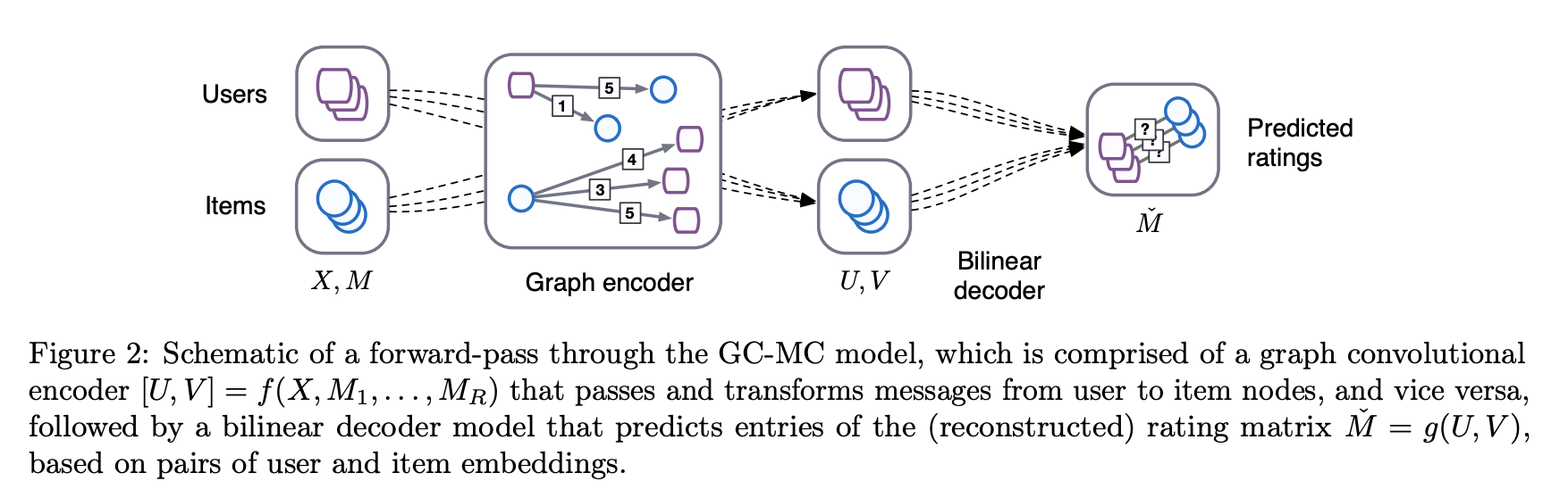 GC-MC forward pass schematic structure. From original paper
Training iGC-MC
We train this graph auto-encoder by minimising the log likelihood of the predicted ratings $\hat{A}_{ij}$. Unlike with explicit feedback, our loss is not only calculated over observed user-item pairs in $\mathcal{O}$. In the implicit feedback setting we need to account for the binary nature of interactions by sampling a number of negative user-item pairs from $\mathcal{O}^-$. The number of negative samples per positive sample is an integer hyperparameter $c$. We call this combined set of positive and negative samples $\mathcal{S}$. Thus our objective function, equivalent to a binary cross-entropy loss, which we seek to minimise is:
\[\begin{aligned} \mathcal{L} &= -\sum_{u,i \in \mathcal{S}} p_{ui} \log{\hat{a}_{ui}} + (1-p_{ui})\log{(1-\hat{a}_{ui})} \end{aligned}\]where $p_{ui} \in {0,1}$ is the true interaction between user $u$ and item $i$, whilst $\hat{a}_{ui}$ is our model’s output - a probability of interaction.
Node dropout
As a form of regularisation we randomly drop out all outgoing messages of a particular node with probability $p_{\text{dropout}}$ , which we refer to as node dropout. We also employ regular dropout in the fully connected layers of our model. The original GC-MC authors note that node dropout served as a better regulariser than message dropout, whereby outgoing messages are dropped out independently making the model more robust to the absence of single edges that represent a single user-item observation.
## Incorporating side information With our problem setting abstracted into the non-Euclidean domain of a graph, we find a natural way to include a feature vector of side information for each node directly into the input feature matrix. However, as noted by in the original GC-MC paper, when the content information is not rich enough to distinguish different users (or items), this leads to a bottleneck of information flow. In this case you can opt for a different method to include these features that uses a separate processing channel directly into the dense hidden layer.
Suppose item node $i$ has side information vector $y_i^f$. We pass $y_i^f$ through a dense layer to output a vector $f_i \in \mathbb{R}^m$, where $m$ is a hyperparameter. We then concatenate $f_i$ with the intermediate node embedding $h_i$, then passed through a separate dense layer to produce our final node embedding $y_i \in \mathbb{R}^f$. Where previously we had $y_i = \sigma(W’h_i)$, this now becomes:
\[\begin{aligned} y_i = \sigma(W_2[h_i, f_i]) \;\;\; \text{with} \;\;\; f_i = \sigma(W_1 y_i^f + b) \end{aligned}\]with $W_1, W_2, b$ all trainable weight matrices. User nodes, without any side information, are processed through the same dense layer as before with a different parameter matrix than the one used above for the item nodes. In the presence of side information, the initial input feature matrix $O$ is simply chosen as an identity matrix, with a unique one-hot vector for every node in the graph.
From GC-MC to iGC-MC
So there you have the theory for iGC-MC - let’s outline the changes and contributions we made to adapt the original GC-MC method to the implicit feedback setting. These are:
- Using a single edge type and processing channel to model whether that edge represents an interaction between the two nodes it connects (one user, one item). Previously each rating level was given its own processing channel.
- Weigh messages according to their confidence, as given by the weighted average of edges weights incoming to that node.
- Loss function. We change the model output from a score per rating level to a single scalar output, passed through a sigmoid nonlinearity so as to interpret it as the probability of interaction. Accordingly, our loss function became a binary cross-entropy loss vs what was previously a cross-entropy loss, where a softmax had been applied in the original presentation of the method.
- Negative interactions. We sample a number of negative unobserved user-item pairs to contribute to the loss function. Learning would not be possible without this step, since the label of all items contributing to the loss would be positive. These unobserved user-item pairs correspond to `empty’ edges on the graph.
Check out my code base for the model. I’ll be writing a follow up soon on implementing the model against some baselines on a public dataset! Lots of background and things to dig into from this post - some suggestions below.