arXiv-GPT: predicting Machine Learning abstracts

Code & notebook for this post can be found here. Check out Part 1 where we introduce the dataset.

The release of OpenAI’s GPT-3 generated much deserved buzz and excitment in Tech circles and beyond, with main-stream press reporting on the technology - whilst the theory behind the model has been around for several years, the creation of an API, releasing a beta version to some developers, was the real geniuns of the release in my mind.

In this post, we explore a smaller Generative Pretrained Transformer (GPT), based of Andrej Karpathy’s minGPT - a PyTorch re-implementation of OpenAI’s GPT that “tries to be small, clean, interpretable and educational” (it is.) We take all the abstracts from papers in the fields of Machine Learning and Ariticial Intelligence from the arXiv dataset on Kaggle (which provides meta-data on thousands of papers published over the past decade). Our GPT is then trained on those abstracts on a single GPU available on Google Colabatory notebook.

Finally, we feed our trained model some prompts to predict an entire Machine Learning abstract. Sneak preview of our (fairly coherent) results below!

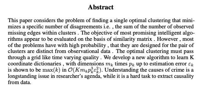
Sampled abstract from the prompt ‘This paper considers…’. Formatted in LaTeX with the NeurIPS template for fun :)

Setup

First the boring stuff - to import your own packages in a Google Colab you need to mount your own drive and cd into the right folder.

from google.colab import drive # import drive from google colab

ROOT = "/content/drive"     # default location for the drive
print(ROOT)                 # print content of ROOT (Optional)

drive.mount(ROOT)           # we mount the google drive at /content/drive

# This is necessary to ensure that paths are correct for importing data from the google drive folder
# insert correct root for minGPT code
minGPT_DIR = '/minGPT/'
%cd $minGPT_DIR

Next up, we follow the set-up used in the character-level GPT example online importing necessary modules.

# set up logging
import logging
logging.basicConfig(
        format="%(asctime)s - %(levelname)s - %(name)s -   %(message)s",
        datefmt="%m/%d/%Y %H:%M:%S",
        level=logging.INFO,
)

# make deterministic
from mingpt.utils import set_seed
set_seed(42)

import numpy as np
import torch
import torch.nn as nn
from torch.nn import functional as F

import re
import numpy as np 
import pandas as pd
import os
import json
pd.set_option('float_format', '{:f}'.format)

Data

Let’s load the data, using yield below to avoid memory problems with the huge json file.

file_path = 'arxiv-metadata-oai-snapshot.json'

def get_metadata():
    with open(file_path, 'r') as f:
        for line in f:
            yield line

We’ll just look at papers from the past 10 years and select those part of the three categories arXiv tags AI papers in:

• cs.AI: Artificial Intelligence
• cs.LG: Machine Learning
• stat.ML: Machine Learning

That gets us 4673 abstracts to work with!

ai_list = ['cs.AI','cs.LG','stat.ML']
abstracts = []

metadata = get_metadata()
# loop over all papers
for paper in metadata:
    # extract single paper
    paper_dict = json.loads(paper)
    version = paper_dict.get('versions')
    category = paper_dict.get('categories')
    try:
        try:
            year = int(paper_dict.get('journal-ref')[-4:])    ### Example Format: "Phys.Rev.D76:013009,2007"
        except:
            year = int(paper_dict.get('journal-ref')[-5:-1])    ### Example Format: "Phys.Rev.D76:013009,(2007)"

        if any(ele in category for ele in ai_list) and 2010<year<2021:
            abstracts.append(paper_dict.get('abstract'))
    except:
        pass

len(abstracts)

4673

Next we need to preprocess the abstracts into one large chunk of text to build an appropriate data object for our GPT model. After these steps we get a corpus of 857,479 words.

# string whitespace at end of words, replace new lines by space and add 'end of sentence' token
f = lambda x: x.strip().replace("\n"," ") + " #EOS"
abstracts = [f(x) for x in abstracts]
# seperate all words and punctuation
abstracts = [re.findall(r"[\w']+|[.,!?;]", x) for x in abstracts]
# turn list of lists in to single list
abstracts = [j for i in abstracts for j in i]

len(abstracts)

857479

Now we’re ready to build our Dataset object - taking almost the same form as the character-level dataset as before, but changing our vocab and look-ups as needed.

import math
from torch.utils.data import Dataset

class WordDataset(Dataset):

    def __init__(self, data, block_size):
        words = sorted(list(set(data)))
        data_size, vocab_size = len(data), len(words)
        print('data has %d words, %d unique.' % (data_size, vocab_size))
        
        self.stoi = { ch:i for i,ch in enumerate(words) }
        self.itos = { i:ch for i,ch in enumerate(words) }
        self.block_size = block_size
        self.vocab_size = vocab_size
        self.data = data
    
    def __len__(self):
        return len(self.data) - self.block_size

    def __getitem__(self, idx):
        # grab a chunk of (block_size + 1) characters from the data
        chunk = self.data[idx:idx + self.block_size + 1]
        # encode every word to an integer
        dix = [self.stoi[s] for s in chunk]
        """
        # See https://github.com/karpathy/minGPT/blob/master/play_char.ipynb for
        # explainer of Dataset construction
        """
        x = torch.tensor(dix[:-1], dtype=torch.long)
        y = torch.tensor(dix[1:], dtype=torch.long)
        return x, y

With our Dataset object defined we can load our dataset with a block size of 128 appropriate since the average abstract in arXiv 122 words long (see prev post).

block_size = 128 # sets spatial extent of the model for its context
train_dataset = WordDataset(abstracts, block_size) 

data has 857479 words, 25921 unique.

Training

Let’s load a GPT! In the character-level transformer example Karpathy built a ‘GPT-1’ with 8 layers and 8 heads - here we halve that to 4 layers and 4 attention heads so to able to train it on the memory available with a Colab GPU (I guess we call this ‘GPT-0.5’…)

from mingpt.model import GPT, GPTConfig
mconf = GPTConfig(train_dataset.vocab_size, train_dataset.block_size,
                  n_layer=4, n_head=4, n_embd=256)
model = GPT(mconf)

09/27/2020 19:49:54 - INFO - mingpt.model -   number of parameters: 1.646387e+07

Training loop with a slightly smaller batch-size.

from mingpt.trainer import Trainer, TrainerConfig

# initialize a trainer instance and kick off training
tconf = TrainerConfig(max_epochs=2, batch_size=128, learning_rate=6e-4,
                      lr_decay=True, warmup_tokens=256*20, final_tokens=2*len(train_dataset)*block_size,
                      num_workers=4)
trainer = Trainer(model, train_dataset, None, tconf)
trainer.train()

epoch 1 iter 6698: train loss 1.35257. lr 3.000110e-04: 100%|██████████| 6699/6699 [24:41<00:00,  4.52it/s]
epoch 2 iter 6698: train loss 0.94379. lr 6.000000e-05: 100%|██████████| 6699/6699 [24:45<00:00,  4.51it/s]

Sampling

Model trained! Let’s generate some Machine Learning abstracts…

1)

# alright, let's sample some word-level abstracts
from mingpt.utils import sample

context = ['This', 'paper', 'discusses']
x = torch.tensor([train_dataset.stoi[s] for s in context], dtype=torch.long)[None,...].to(trainer.device)
y = sample(model, x, 150, temperature=1.0, sample=True, top_k=10)[0]
completion = ' '.join([train_dataset.itos[int(i)] for i in y])
print(completion)

This paper discusses the effect of the design and implementation of a case study . Graph Neural Networks GNNs achieve remarkable performance in graph data classification tasks . In graph classification , each node of node information from labeled nodes measured nodes in a graph are connected by many , each graph represents the goal of node embedding space . Multiple graph embedding aims to create a similarity graph by representing the different graph each path graph in each graph . This information represents the embedding by learning a knowledge graph by node as the network . The goal is to design a similarity graph embedding that represents a set of entities and the entities in the graph . The nodes are generated using graph embedding techniques , which represent graph embedding methods with embedding methods , on nodes using graphs .

2)

context = ['Our', 'work', 'has', 'focused', 'on']
x = torch.tensor([train_dataset.stoi[s] for s in context], dtype=torch.long)[None,...].to(trainer.device)
y = sample(model, x, 200, temperature=1.0, sample=True, top_k=10)[0]
completion = ' '.join([train_dataset.itos[int(i)] for i in y])
print(completion)

Our work has focused on the use of multi modal social networks and web recommender systems , in which contain heterogeneous information and items . In this paper , we propose a multi modal data embedding framework to detect matches semantically similar contexts in order to their opinions . We show that both methods can be successfully applied to Web and document clustering tasks . EOS In this paper we study the problem of finding the rating of two and , the rating score for a given time . In particular , we use the following the following questions 1 The given answer is a certain item such that the set of at any a certain item we choose one , and use the rating , combined with the answer to answer based . We review the characteristics and compare the baselines in detail to these questions . To this end , we built a deep ranking approach for general and general and statistical analysis of some recent QA methods . EOS We consider the problem of learning a probabilistic domain , agent using data . Given a collection of Chinese e commerce , we allow a posterior over a subset of interest , and

3)

context = ['This', 'paper', 'considers']
x = torch.tensor([train_dataset.stoi[s] for s in context], dtype=torch.long)[None,...].to(trainer.device)
y = sample(model, x, 150, temperature=1.0, sample=True, top_k=10)[0]
completion = ' '.join([train_dataset.itos[int(i)] for i in y])
print(completion)

This paper considers the problem of finding a single optimal clustering that minimizes a specific number of disagreements i . e . , the sum of the number of observed missing edges within clusters . The objective of most promising intelligent algorithms appear to be evaluated on the basis of similarity matrix . However , most of the problems have with high probability , that they are designed for the pair of clusters are distinct from observational data . The optimal clustering must pass through a grid like time varying quality . We develop a new algorithm to learn K coordinate dictionaries , with dimensions m_k times p_k up to estimation error varepsilon_k is shown to be max_ k in K mathcal O m_kp_k 3 varepsilon_k 2 . Understanding the causes of crime is a longstanding issue in researcher’s agenda , while it is a hard task to extract causality from data

Not bad for a small-ish model (10m vs 160bn for a full GPT-3!) on less than an hour training! What worked and what didn’t?

• Topics are current and relevant (expected) - GNNs, reecommender systems…
• Most sentences are coherent.
• Example 3 managed to get some maths in there even mentioning the time complexity of the paper’s method which certainly impressed me.
• EOS and punctuation a bit all over the place.
• Abstracts aren’t always consistent on a topic from start to finish.

Conclusion

The success of GPT-3 has spun up a lot of debate as to whether these enormous language models have an ‘understanding’ of words, know what concepts mean and can reason. Some say it doesn’t matter and for a lot of purposes I agree, it doesn’t. However when discussing AGI, I think it does and even with GPT-3 you don’t have to look too far to ‘fool’ it. What our little experiment above shows is that a GPT can pick up corelations in the text at many different levels - each layer or set of attention heads may learn relations between words or even ‘concepts’, style, grammar, maths and more - if it is there in the text. But these models can’t go further than what might be in the text for now…

Lastly, minGPT is a really outstanding resource for learning about transformers - understanding the theory is one thing but then seeing it coded can often be completely different and you gain a lot from seeing a big model like this broken down so well. Plus, a bonus is that its in PyTorch!