arXiV: a rudimentary EDA

Check out the notebook for this post here

In this post we’re going to perform a straightforward Exploratory Data Analysis (EDA) on a dataset; whereby we load it, perform some sensible preprocessing steps, generate some statistics to get a sense of the data then answer some more interesting questions about the dataset with some plots.

The dataset we’re going to examine is the ArXiv dataset from Kaggle, a “repository of 1.7 million articles, with relevant features such as article titles, authors, categories, abstracts, full text PDFs, and more.”

ArXiv provides open access to scholarly articles (such as research papers), so we can do some interesting analysis about the change in interest of, say, AI/ML related articles.

Creating a DataFrame

import numpy as np 
import pandas as pd
import plotly_express as px
import os
import json
pd.set_option('float_format', '{:f}'.format)

Let’s load the data, we use ‘yield’ to get the necessary information in a loop since json files in the dataset are huge so we avoid memory problems.

file_path = 'arxiv-metadata-oai-snapshot.json'

def get_metadata():
    with open(file_path, 'r') as f:
        for line in f:
            yield line

Looking at one example of a paper we see lots of information available: a series of dates in the ‘versions’, author names, an abstract, categories and so on.

metadata = get_metadata()
for paper in metadata:
    for k, v in json.loads(paper).items():
        print(f'{k}: {v}')
    break

id: 0704.0001
submitter: Pavel Nadolsky
authors: C. Bal\'azs, E. L. Berger, P. M. Nadolsky, C.-P. Yuan
title: Calculation of prompt diphoton production cross sections at Tevatron and
  LHC energies
comments: 37 pages, 15 figures; published version
journal-ref: Phys.Rev.D76:013009,2007
doi: 10.1103/PhysRevD.76.013009
report-no: ANL-HEP-PR-07-12
categories: hep-ph
license: None
abstract:   A fully differential calculation in perturbative quantum chromodynamics is
presented for the production of massive photon pairs at hadron colliders. All
next-to-leading order perturbative contributions from quark-antiquark,
gluon-(anti)quark, and gluon-gluon subprocesses are included, as well as
all-orders resummation of initial-state gluon radiation valid at
next-to-next-to-leading logarithmic accuracy. The region of phase space is
specified in which the calculation is most reliable. Good agreement is
demonstrated with data from the Fermilab Tevatron, and predictions are made for
more detailed tests with CDF and DO data. Predictions are shown for
distributions of diphoton pairs produced at the energy of the Large Hadron
Collider (LHC). Distributions of the diphoton pairs from the decay of a Higgs
boson are contrasted with those produced from QCD processes at the LHC, showing
that enhanced sensitivity to the signal can be obtained with judicious
selection of events.

versions: [{'version': 'v1', 'created': 'Mon, 2 Apr 2007 19:18:42 GMT'}, {'version': 'v2', 'created': 'Tue, 24 Jul 2007 20:10:27 GMT'}]
update_date: 2008-11-26
authors_parsed: [['Balázs', 'C.', ''], ['Berger', 'E. L.', ''], ['Nadolsky', 'P. M.', ''], ['Yuan', 'C. -P.', '']]

We now extract a subset of the fields which we will perform our anlysis on.

titles, abstracts, versions, categories, doi, authors_parsed = [], [], [], [], [], []

metadata = get_metadata()
# loop over all papers
for paper in metadata:
    # extract single paper
    paper_dict = json.loads(paper)
    version = paper_dict.get('versions')
    try:
        versions.append(version[-1]['created']) # choose created as the most recent version
        titles.append(paper_dict.get('title'))
        abstracts.append(paper_dict.get('abstract'))
        categories.append(paper_dict.get('categories'))
        doi.append(paper_dict.get('doi'))
        authors_parsed.append(paper_dict.get('authors_parsed'))
    except:
        pass

Let’s create a pandas dataframe to make our analysis easier:

papers = pd.DataFrame({
    'title': titles,
    'abstract': abstracts,
    'categories': categories,
    'version': versions,
    'doi': doi,
    'authors': authors_parsed
})
papers.head()

# reduce memory constraints
del titles, abstracts, versions, categories, doi, authors_parsed

	title	abstract	categories	version	doi	authors
0	Calculation of prompt diphoton production cros...	A fully differential calculation in perturba...	hep-ph	Tue, 24 Jul 2007 20:10:27 GMT	10.1103/PhysRevD.76.013009	[[Balázs, C., ], [Berger, E. L., ], [Nadolsky,...
1	Sparsity-certifying Graph Decompositions	We describe a new algorithm, the $(k,\ell)$-...	math.CO cs.CG	Sat, 13 Dec 2008 17:26:00 GMT	None	[[Streinu, Ileana, ], [Theran, Louis, ]]
2	The evolution of the Earth-Moon system based o...	The evolution of Earth-Moon system is descri...	physics.gen-ph	Sun, 13 Jan 2008 00:36:28 GMT	None	[[Pan, Hongjun, ]]
3	A determinant of Stirling cycle numbers counts...	We show that a determinant of Stirling cycle...	math.CO	Sat, 31 Mar 2007 03:16:14 GMT	None	[[Callan, David, ]]
4	From dyadic $\Lambda_{\alpha}$ to $\Lambda_{\a...	In this paper we show how to compute the $\L...	math.CA math.FA	Mon, 2 Apr 2007 18:09:58 GMT	None	[[Abu-Shammala, Wael, ], [Torchinsky, Alberto, ]]

Preprocessing

As we can see, some columns have different data types, whilst we also have some None or missing values present. The isna() function is helpful to find None or NaN values in data. As an example lets see how many of our papers do not have a DOI:

print('{} of {} papers without DOI'.format(papers['doi'].isna().sum(), len(papers)))

846236 of 1765688 papers without DOI

Now since DOI is often added after a paper is published (source) we won’t remove this column but if we wanted to something such as papers[papers.doi.notnull()] would do the trick.

Next let’s clean up some of the columns:

• We want the abstract to be one continous string of text without new lines.
• versions need to be Python datetime objects then lets extract the month and year they were published.
• The authors column would be better as a list of strings

# clean abstracts
papers['abstract'] = papers['abstract'].apply(lambda x: x.replace("\n",""))
papers['abstract'] = papers['abstract'].apply(lambda x: x.strip())

# extract date time info 
papers['DateTime']= pd.to_datetime(papers['version'])
papers['month'] = pd.DatetimeIndex(papers['DateTime']).month
papers['year'] = pd.DatetimeIndex(papers['DateTime']).year

# clean authors
papers['authors']= papers['authors'].apply(lambda authors:[(" ".join(a)).strip() for a in authors])
papers.head()

	title	abstract	categories	version	doi	authors	DateTime	month	year
0	Calculation of prompt diphoton production cros...	A fully differential calculation in perturbati...	hep-ph	Tue, 24 Jul 2007 20:10:27 GMT	10.1103/PhysRevD.76.013009	[Balázs C., Berger E. L., Nadolsky P. M., Yuan...	2007-07-24 20:10:27+00:00	7	2007
1	Sparsity-certifying Graph Decompositions	We describe a new algorithm, the $(k,\ell)$-pe...	math.CO cs.CG	Sat, 13 Dec 2008 17:26:00 GMT	None	[Streinu Ileana, Theran Louis]	2008-12-13 17:26:00+00:00	12	2008
2	The evolution of the Earth-Moon system based o...	The evolution of Earth-Moon system is describe...	physics.gen-ph	Sun, 13 Jan 2008 00:36:28 GMT	None	[Pan Hongjun]	2008-01-13 00:36:28+00:00	1	2008
3	A determinant of Stirling cycle numbers counts...	We show that a determinant of Stirling cycle n...	math.CO	Sat, 31 Mar 2007 03:16:14 GMT	None	[Callan David]	2007-03-31 03:16:14+00:00	3	2007
4	From dyadic $\Lambda_{\alpha}$ to $\Lambda_{\a...	In this paper we show how to compute the $\Lam...	math.CA math.FA	Mon, 2 Apr 2007 18:09:58 GMT	None	[Abu-Shammala Wael, Torchinsky Alberto]	2007-04-02 18:09:58+00:00	4	2007

Analysis

Looking at each paper, we might want to know things such as how many categories does each paper have? How many words is in the abstract? How many authors are in this paper? Pandas makes this easy with the apply method where you can apply an arbitrary function to produce a new column from another, as below.

papers['num_categories'] = papers['categories'].apply(lambda x:len(x)).astype('int')
papers['num_words_abstract'] = papers['abstract'].apply(lambda x:len(x.split())).astype('int')
papers['num_authors'] = papers['authors'].apply(lambda x:len(x)).astype('int')
papers.head()

	title	abstract	categories	version	doi	authors	DateTime	month	year	num_categories	num_words_abstract	num_authors
0	Calculation of prompt diphoton production cros...	A fully differential calculation in perturbati...	hep-ph	Tue, 24 Jul 2007 20:10:27 GMT	10.1103/PhysRevD.76.013009	[Balázs C., Berger E. L., Nadolsky P. M., Yuan...	2007-07-24 20:10:27+00:00	7	2007	6	127	4
1	Sparsity-certifying Graph Decompositions	We describe a new algorithm, the $(k,\ell)$-pe...	math.CO cs.CG	Sat, 13 Dec 2008 17:26:00 GMT	None	[Streinu Ileana, Theran Louis]	2008-12-13 17:26:00+00:00	12	2008	13	105	2
2	The evolution of the Earth-Moon system based o...	The evolution of Earth-Moon system is describe...	physics.gen-ph	Sun, 13 Jan 2008 00:36:28 GMT	None	[Pan Hongjun]	2008-01-13 00:36:28+00:00	1	2008	14	133	1
3	A determinant of Stirling cycle numbers counts...	We show that a determinant of Stirling cycle n...	math.CO	Sat, 31 Mar 2007 03:16:14 GMT	None	[Callan David]	2007-03-31 03:16:14+00:00	3	2007	7	32	1
4	From dyadic $\Lambda_{\alpha}$ to $\Lambda_{\a...	In this paper we show how to compute the $\Lam...	math.CA math.FA	Mon, 2 Apr 2007 18:09:58 GMT	None	[Abu-Shammala Wael, Torchinsky Alberto]	2007-04-02 18:09:58+00:00	4	2007	15	35	2

We’re now ready to ask some questions about the data, each which can be answered in a few lines of code:

1. How many authors to papers have?

Here we use the describe() method to get a high level summary of the column in question, where a histogram isn’t necessary at this point. We see that most papers have 4 authors or less but there’s a heavy right tail with some papers having a few thousand others. Odd.

papers['num_authors'].astype('int').describe()

count   1765688.000000
mean          4.153911
std          20.305943
min           1.000000
25%           2.000000
50%           3.000000
75%           4.000000
max        2832.000000
Name: num_authors, dtype: float64

Let’s look into the heavy tail a bit more - we see that the top 3 papers with most authors are in the ‘hep-ex’ cateogory which stands for ‘High Energy Physics - Experiment’. If we read the abstract of the most authored paper we see in fact its the result from an experiment Large Hadron Collider at CERN, the product of worldwide scientific collaboratin (and so making sense of the 2832 authors!)

papers.sort_values(by='num_authors', ascending=False).head()

	title	abstract	categories	version	doi	authors	DateTime	month	year	num_categories	num_words_abstract	num_authors
574385	Observation of the rare $B^0_s\to\mu^+\mu^-$ d...	A joint measurement is presented of the branch...	hep-ex hep-ph	Mon, 17 Aug 2015 15:53:53 GMT	10.1038/nature14474	[CMS The, Collaborations LHCb, :, Khachatryan ...	2015-08-17 15:53:53+00:00	8	2015	13	99	2832
101754	Expected Performance of the ATLAS Experiment -...	A detailed study is presented of the expected ...	hep-ex	Fri, 14 Aug 2009 13:50:42 GMT	None	[The ATLAS Collaboration, Aad G., Abat E., Abb...	2009-08-14 13:50:42+00:00	8	2009	6	80	2612
535194	The Physics of the B Factories	This work is on the Physics of the B Factories...	hep-ex hep-ph	Sat, 31 Oct 2015 06:42:11 GMT	10.1140/epjc/s10052-014-3026-9	[Bevan A. J., Golob B., Mannel Th., Prell S., ...	2015-10-31 06:42:11+00:00	10	2015	13	111	2034
901222	Search for High-energy Neutrinos from Binary N...	The Advanced LIGO and Advanced Virgo observato...	astro-ph.HE	Thu, 9 Nov 2017 05:44:40 GMT	10.3847/2041-8213/aa9aed	[Albert A. ANTARES, IceCube, Pierre\n Auger,...	2017-11-09 05:44:40+00:00	11	2017	11	170	1945
1041880	Search for Multi-messenger Sources of Gravitat...	Astrophysical sources of gravitational waves, ...	astro-ph.HE	Thu, 15 Nov 2018 21:37:04 GMT	10.3847/1538-4357/aaf21d	[ANTARES, IceCube, LIGO, Collaborations Virgo,...	2018-11-15 21:37:04+00:00	11	2018	11	133	1595

papers.iloc[574385]['abstract'][:250]

'A joint measurement is presented of the branching fractions$B^0_s\\to\\mu^+\\mu^-$ and $B^0\\to\\mu^+\\mu^-$ in proton-proton collisions at theLHC by the CMS and LHCb experiments. The data samples were collected in 2011 ata centre-of-mass energy of 7 TeV, '

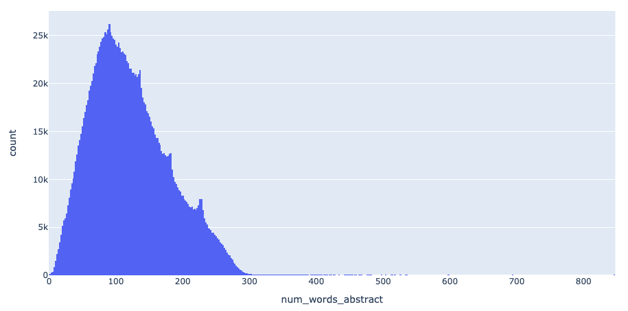
2. How many words does the average abstract have?

Next lets look at how abstracts are in general, where a histogram will be a good option to visualise the data. As expected most aren’t too long with the average abstract 122 words long.

fig = px.histogram(papers, x="num_words_abstract", nbins=500)
fig.show()

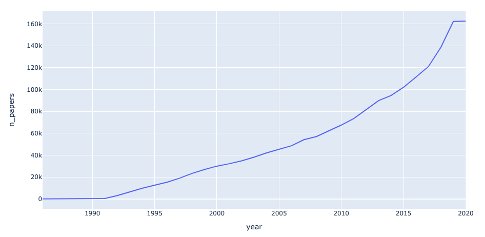
3. How many papers have been produced over time?

We plot a line chart to answer this question. To count the number of papers per year, we used the groupby() method, a powerful tool in pandas to aggregate information in a large variety of ways.

There’s a steady growth of papers published over time as ArXiV became more popular and wide reaching, whilst also perhaps reflecting the higher output of research in Science across the world. Since we’re half way through 2020 the line tails off as expected. This makes sense.

papers_per_year = papers.groupby(['year']).size().reset_index().rename(columns={0:'n_papers'})
fig = px.line(x='year', y='n_papers', data_frame=papers_per_year)
fig.show()

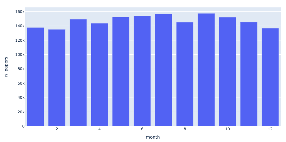
4. In which months are the most papers published?

We see little variation across months excpet a slight decrease across Winter and Christmas months, but nothing significant.

papers_per_month = papers.groupby(['month']).size().reset_index().rename(columns={0:'n_papers'})
fig = px.bar(x='month', y='n_papers', data_frame=papers_per_month)
fig.show()

## AI & ML

Now let’s filter for papers related to AI & ML. It’s not as simple as using papers['categories'].isin(ai_list) since most papers have more than one categories. So we use the intermediate step of seeing if any of the categories of the paper are in the first. If at least one is in the list we assign a value of True to this intermediate variable and filter for values. Note this could have been done in a single line but for clarity we split this out.

ai_list=['cs.AI','cs.LG','stat.ML']
papers['is_ai'] = papers['categories'].apply((lambda x: any(ele in x for ele in ai_list)==True))
ai_papers = papers[papers['is_ai']==True]
ai_papers.head()

	title	abstract	categories	version	doi	authors	DateTime	month	year	num_categories	num_words_abstract	num_authors	is_ai
46	Intelligent location of simultaneously active ...	The intelligent acoustic emission locator is d...	cs.NE cs.AI	Sun, 1 Apr 2007 13:06:50 GMT	None	[Kosel T., Grabec I.]	2007-04-01 13:06:50+00:00	4	2007	11	155	2	True
49	Intelligent location of simultaneously active ...	Part I describes an intelligent acoustic emiss...	cs.NE cs.AI	Sun, 1 Apr 2007 18:53:13 GMT	None	[Kosel T., Grabec I.]	2007-04-01 18:53:13+00:00	4	2007	11	124	2	True
303	The World as Evolving Information	This paper discusses the benefits of describin...	cs.IT cs.AI math.IT q-bio.PE	Wed, 13 Oct 2010 19:49:16 GMT	10.1007/978-3-642-18003-3_10	[Gershenson Carlos]	2010-10-13 19:49:16+00:00	10	2010	28	107	1	True
670	Learning from compressed observations	The problem of statistical learning is to cons...	cs.IT cs.LG math.IT	Thu, 5 Apr 2007 02:57:15 GMT	10.1109/ITW.2007.4313111	[Raginsky Maxim]	2007-04-05 02:57:15+00:00	4	2007	19	138	1	True
953	Sensor Networks with Random Links: Topology De...	In a sensor network, in practice, the communic...	cs.IT cs.LG math.IT	Fri, 6 Apr 2007 21:58:52 GMT	10.1109/TSP.2008.920143	[Kar Soummya, Moura Jose M. F.]	2007-04-06 21:58:52+00:00	4	2007	19	244	2	True

As before lets try and answer some questions about this subset of the data.

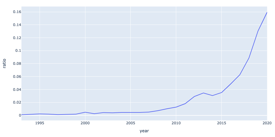
5. What is the growth of of AI & ML papers published over the years?

For this we need to count both the total number of papers published each year as well as the total number of AI & ML papers published each year; then we compare the two and plot the result. As before we use the groupby() method on the main and smaller dataframes, then use merge() to compare the two.

The plot shows an exponential growth in the topic kicking off around 2006, around the time ImageNet was released with several other seminal papers contributing to this explosion of growth.

# total papers published per year
all_papers_per_year = papers.groupby(['year']).size().reset_index().rename(columns={0:'all'})
# AI & ML papers published per year
ai_papers_per_year = ai_papers.groupby(['year']).size().reset_index().rename(columns={0:'AI'})

# merge and calculate percentage
compare = all_papers_per_year.merge(ai_papers_per_year, how='inner')
compare['ratio'] = compare['AI']/compare['all']

# plot
fig = px.line(x='year', y='ratio', data_frame=compare)
fig.show()

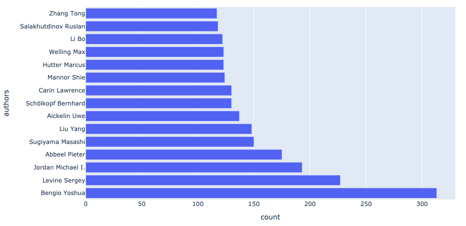
6. Which authors have published the most work?

Yoshua Bengio, one of the fathers of Deep Learning, comes top of the list with over 300 papers published in our dataset! An impressive number.

# flatten list of authors
authors = [y for x in ai_papers['authors'].tolist() for y in x]
authors_df = pd.DataFrame({'authors': authors}).groupby(['authors']).size().reset_index().rename(columns={0:'count'})
authors_df = authors_df.sort_values('count',ascending=False).head(15)
# plot
fig = px.bar(x='count', y='authors', data_frame=authors_df)
fig.show()

Conclusion

There you have a quick intro to EDA with some useful methods in pandas that help you along your way. Its always important to understand your dataset before diving into a Machine Learning model and asking + answering some high level questions is a good way to start. Your data should always inform your model choices and make you think about what to try and why.

Find the notebook for this post here