Evaluating Word Embeddings

For an introduction to word embeddings and why sparsity is important check out my previous post here.

So you’ve got a set of word embeddings, sparse or dense, trained by some deep learning algorithm such as skip-gram or CBOW - how do you figure out if they’re any good? Well, we generally care about three things when assessing the quality of word embeddings:

• Interpretability, for example, are the embedding dimensions coherent?
• Expressive power, for example, is the similarity between words captured?
• Performance on downstream language tasks, for example, sentiment analysis or question-answering.

Whilst a human-in-the-loop often provides the only true answer to these often questions, there do exist quantitative ways of measuring these qualities used in literature. The section that follows detail tests used to evaluate the interpretability (word intrusion) and expressive power (word similarity and word analogy).

Word Intrusion

Take your matrix of embeddings of size $|\mathcal{V}| \times d$, where each word embedding in your vocabulary of size $|\mathcal{V}|$ has size $d$. For each dimension $i$ of the learned word vector, we sort the word embeddings in descending order on that dimension alone. Next, we create a set of the top $5$ words from the sorted list and randomly sample one word from the bottom half of the list that is also present in the top $10\%$ of another dimension $i’$. The word added from the bottom half of the sorted list is referred to as an \textit{intruder}. An example of such a set is shown below:

{poisson, parametric, markov, bayesian, stochastic, jodel}

where jodel is clearly the intruder word, describing an aircraft company, while the rest of the words represent various statistical concepts.

Standard word intrusion uses a human judge to identify the intruder word. However, we use the automatic metric proposed by 1 that captures the intuition of the task without needing manual assessment: “the intruder word should be dissimilar to the top 5 words while those top words should be similar to each other.” We measure the ratio of the distance between the intruder word and top words to the distance between the top words themselves. A higher ratio corresponds to better interpretability since it indicates that the intrusion word is far away from the top words in embedding space and so can be easily identified. Formally we calculate:

\[\begin{aligned} DistRatio &= \frac{1}{d} \sum_{i=1}^d \frac{InterDist_i}{IntraDist_i} \\ InterDist_i &= \sum_{w_j \in top_i(i)} \frac{dist(w_j, w_{b_i})}{k} \\ IntraDist_i &= \sum_{w_j \in top_k(i)} \sum_{w_k \in \mathrm{top}_k(i), w_k \neq w_j} \frac{\mathrm{dist}(w_j, w_{k})}{k(k-1)} \end{aligned}\]

where $top_k(i)$ is the top $k$ words on dimension $i$, $w_{b_i}$ is the intrusion word for dimension $i$ and $\mathrm{dist}(w_j, w_k)$ denotes the Euclidean distance between word $w_j$ and $w_k$. $\mathrm{IntraDist}_i$ is the average distance between the top $k$ words in dimension $i$ and $\mathrm{InterDist}_i$ denotes the average distance between the intruder word and top words on that dimension. We set $k=5$ and average the result over ten runs since there is stochasticity in the selection of intruder words.

Word Similarity

The first of two tasks that evaluate the expressive power of our learnt word embeddings is word similarity. The task measures how well the learnt embeddings capture similarity between words. Two datasets most often used for this are WordSim-$353$ and SimLex-$999$, the second of which is constructed to overcome the shortcomings of WordSim-$353$. SimLex contains $999$ pairs of nouns ($666$), verbs ($222$), and adjectives ($111$) each with a human annotated similarity score. The cosine angle between the embedding representation of each pair of words is calculated and we report the spearman rank correlation coefficient $\rho_{sim}$ between the calculated cosine angles and the list of human scores.

For example the pair of words coast - shore have a Simlex-$999$ score of $9.00$. We hope that the embedding vector also share a high degree of similarity.

Word Analogy

The word analogy task consists of analogies of the form “a is to b as c is to ?”. The goal of the task, given a tuple of words (a, b, c, d) and corresponding word vectors ($w_a, w_b, w_c$), is to correctly identify the missing word. We measure whether the model correctly identifies the missing word by calculating $w_d = w_b - w_a + w_c$ and finding the word vector in the vocabulary that is closest to $w_d$ in cosine distance, with only an exact match counting as success.

A common dataset used for this task is that from the original Word2Vec paper called the `questions-words’ dataset, which consists of $19,544$ tuples.

Other

Downstream tasks: Once scores for the above three tasks have been collected you can turn to extrinsic evaluation i.e. feedings your embeddings into a larger model used for a downstream language task and seeing how well the overall model does. To assess the impact of a different set of embeddings, simply keep your experimental setup exactly the same and change the set of embeddings used in the model.

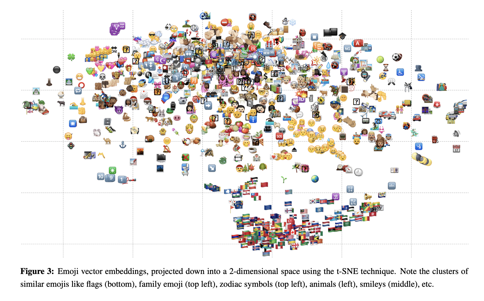
Visualisation: A final mention for the much-loved t-SNE technique, which allows us to visualise our embeddings in $2$D or $3$D. t-SNE creates a low-dimensional representation of high-dimensional input data while preserving distances between similar points in the original input space. Its often used in the context of embeddings to qualitatively assess if groups of objects share a similar region in the projected subspace. A fun example below is from the emoji2vec paper where flags, animals, family emojis appear in clusters.

---

To see an implementation of the three intrinsic tasks in Python be sure to check out our repo embedtrics here