
Visualising CNN feature-maps and layer activations
Convolutional Neural Networks are the most successful deep learning architecture for Computer Vision tasks, particularly image classification. They comprise of a stack of Convolutional layers, Pooling layers and Fully-connected layers, which combine.
We build a simple Convolutional Neural Network in PyTorch, trained to recognise hand-written digits using the MNIST dataset and focus on examining the Convolutional layers. The pooling layers make the model translational invariant - something clearly important in Computer Vision.
Each filter, or kernel, learns a particular feature of the dataset. After passing over an image, a filter produces a feature map which we can visualise. In this post, I’ll explain how to produce the following visualisations of our CNN layers, helping us to interpret our model better:
- Feature map for each convolutional layer, showing activations for a single image.
- Average activations of each Feature over the entire training set.
- Histogram of average activations of each Feature.
import os
import numpy as np
import matplotlib.pyplot as plt
%matplotlib inline

import torch
import torchvision
from torchvision import datasets, models, transforms
import torch.nn as nn
import torch.nn.functional as F
import torch.optim as optim
from torch.utils.data import DataLoader

device = torch.device("cuda" if torch.cuda.is_available() else "cpu")
print(device)

# set seeds
np.random.seed(0)
torch.manual_seed(0)
Loading our Data
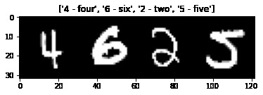
MNIST consists of 70,000 greyscale 28x28 images (60,000 train, 10,000 test). We use inbuilt torchvision functions to create our DataLoader objects for the model in two stages:
-
Download the dataset using
torchvision.datasets. Here we can transform the data, turning it into a tensor and normalising the greyscale values with zero mean and unit standard deviation (the values 0.1307 and 0.3081 are the global mean/std for the MNIST images, these will be different according to your dataset). Since our images are already centered we need no more preprocessing but there’s a whole suite of transformations available here such asRandomHorizontalFlip,CenterCrop,Scaleto name a few. -
Create a
DataLoaderfrom the Datasets object, with a different batch size for training and validation (larger since more examples can be processed in parallel at inference time).
We also store the class names and lablels, for use later.
# set transformations
transformations = transforms.Compose([
        transforms.ToTensor(),
        transforms.Normalize((0.1307,), (0.3081,))
        ])

# inputs into Datasets object
root_dir = '../visual_cnn/data/'
download_train= {'train': True, 'val': False}
batch_size = {'train': 256, 'val': 1024}

# create train and validation Datasets object
image_datasets = {x: torchvision.datasets.MNIST(root=root_dir+'/'+x+'/',
                                                train=download_train[x],
                                                transform=transformations,
                                                download=True) for x in ['train', 'val']}

# create DataLoader objects
dataloaders = {x: torch.utils.data.DataLoader(image_datasets[x],
                                              batch_size=batch_size[x],
                                              shuffle=True) for x in ['train', 'val']}

# get class names
class_names = image_datasets['train'].classes
class_labels = list(image_datasets['train'].class_to_idx.values())
print(class_names)
['0 - zero', '1 - one', '2 - two', '3 - three', '4 - four', '5 - five', '6 - six', '7 - seven', '8 - eight', '9 - nine']
Lets view some sample images from the dataset.
def imshow(inp, title=None):
    """Imshow for Tensor."""
    inp = inp.numpy().transpose((1, 2, 0))
    inp = np.clip(inp, 0, 1)
    plt.imshow(inp)
    if title is not None:
        plt.title(title)
    plt.pause(0.001)  # pause a bit so that plots are updated

# Get a batch of training data
inputs, classes = next(iter(dataloaders['train']))

# Make a grid from batch
out = torchvision.utils.make_grid(inputs[:4])

imshow(out, title=[class_names[x] for x in classes[:4]])
Constructing our model
Now we can build our CNN class: we use two convolutional layers each followed by a max pooling layer, the outputs of which are fed into a three-layer MLP for classification. Our hyperparameter settings for the kernel size, stride and padding ensure that the input and output dimensions of each image match. See these notes for more details. The pooling layers reduce each image dimensions by half, applied twice, so the input to our MLP has dimesnions 16 x 7 x 7 (where 16 is the number of out channels of our second convolutional layer). Dropout at each layer helps to avoid overfitting, by randomly shutting off parameters with probability given as the dropout parameter.
class CNN(nn.Module):
    def __init__(self, dropout=0, dropout2d=0):
        super(CNN, self).__init__()
        self.conv1 = nn.Conv2d(in_channels=1, out_channels=6, kernel_size=3, padding=1)
        self.pool = nn.MaxPool2d(2, 2)
        self.conv2 = nn.Conv2d(in_channels=6, out_channels=16, kernel_size=3, padding=1)
        self.fc1 = nn.Linear(16 * 7 * 7, 120)
        self.fc2 = nn.Linear(120, 84)
        self.fc3 = nn.Linear(84, 10)
        self.Dropout = nn.Dropout(p=dropout)
        self.Dropout2d = nn.Dropout2d(p=dropout2d)

    def forward(self, x):
        # first convolutional layer
        x = self.Dropout2d(self.pool(F.relu(self.conv1(x))))
        # second convolutional layer
        x = self.Dropout2d(self.pool(F.relu(self.conv2(x))))
        x = x.view(-1, 16 * 7 * 7)
        x = self.Dropout(F.relu(self.fc1(x)))
        x = self.Dropout(F.relu(self.fc2(x)))
        x = self.fc3(x)
        return x
We now define some helper functions. First one to save our model parameters when instructud (that which minimises the validation loss).
def save_checkpoint(state, ep, filename='checkpoint.pth.tar'):
    """Save checkpoint if a new best is achieved"""
    print("=> Saving a new best at epoch:", ep)
    torch.save(state, filename)  # save checkpoint
Next we define our training function. This is a generic PyTorch trainer for any nn.Module, that will accept the usual training parameters (optimiser, DataLoader, epochs) and return the trained model plus your losses and accuracies.
def train(model, lossFun, optim, scheduler, n_epochs, train_loader, val_loader, saveModel=False, verbose=False):
    """Train CNN model"""

    print("Summary of model\n")
    print(model)
    print("\n")

    # initialize lists to store loss and accuracy
    trainLossVec , valLossVec, trainAccuracyVec, valAccuracyVec = [], [], [], []
    bestLoss, bestEpoch = 100, 0

    # get number of batches
    numberBatches = len(train_loader)

    for epoch in range(n_epochs):

        # Set model to training mode
        model.to(device)
        model.train()

        # Loop over each batch from the training set
        for batch_idx, (inputs, targets) in enumerate(train_loader):

            # Zero gradient buffers
            optim.zero_grad()
            # Foward pass and compute loss on batch
            outputs = model(inputs.to(device))
            batchloss = lossFun(outputs, targets.long().to(device)) #commen
            # Backpropagate and update weights
            batchloss.backward()
            # gradient clipping
            torch.nn.utils.clip_grad_norm_(m.parameters(), 1., norm_type=2)
            # optimizer step
            optim.step()

        # set model to evaluation mode
        model.eval()
        with torch.no_grad():
            # evaluate model on training and validation data
            acc, loss = evaluate(model, {"train": train_loader, "val": val_loader}, lossFun)
            # update accuracy
            trainAccuracyVec.append(acc["train"])
            valAccuracyVec.append(acc["val"])
            # update loss
            trainLossVec.append(loss["train"])
            valLossVec.append(loss["val"])

            if scheduler != None:
                scheduler.step()

            # check if new best for validation accuracy
            if valLossVec[-1] < bestLoss:
                bestLoss = valLossVec[-1]
                bestEpoch = epoch
                if saveModel == True:
                    torch.save(m.state_dict(), "bestModel.pt")
                    print("New best value for validation loss: Saved model to bestModel.pt")

            # print information about training progress
            if verbose == True:
                print(("Epoch: {} \t Loss (train): {:.3f} (val): {:.3f} \t" +
              "Acc (train) {:.3f} (val): {:.3f}").format(epoch + 1,
                            trainLossVec[-1], valLossVec[-1], trainAccuracyVec[-1], valAccuracyVec[-1]))
            # clean up
            del inputs, targets, outputs, acc, loss

    return trainLossVec, valLossVec, trainAccuracyVec, valAccuracyVec, bestEpoch
Finally we define a function that calculates the loss + accuracy of our model, which helps make our training loop cleaner.
def evaluate(model, dataDict, lossFun):
    """Calculate loss + accuracy of specified Dataloaders"""
    # extract data objects
    keys = list(dataDict.keys())
    values = [0] * len(keys)

    acc = dict(zip(keys, values))
    lossDict = dict(zip(keys, values))

    # set model to evaluate model
    model.to(device)
    model.eval()
    # stop tracking gradients
    with torch.no_grad():
        # loop over specified dataloaders
        for data in dataDict.keys():
            lossVal = 0
            correct = 0

            for (inputs, targets) in dataDict[data]:
                batchsize = len(targets)
                outputs = model(inputs.to(device))

                # times by batchsize to scale up total loss correctly
                lossVal += lossFun(outputs, targets.long().to(device)).item()*batchsize
                _, pred = torch.max(outputs.data, 1)
                correct += (pred == targets.long().to(device)).sum().item()

            # store values
            lossVal = lossVal/len(dataDict[data].dataset)
            accuracy = correct/len(dataDict[data].dataset)
            acc[data] = accuracy * 100
            lossDict[data] = lossVal

            # clean up
            del inputs, targets, outputs

    return acc, lossDict
Train Model
We’re now ready to train our model! Our task of multi-class classification lends itself to a cross-entropy loss - PyTorch attaches a softmax layer to your model when this loss is used. We use AdamW as our optimiser and use a scheduler to taper the learning rate.
model = CNN(0.1, 0.1)
lr = 1e-03
loss_function = nn.CrossEntropyLoss()
optimiser = optim.AdamW(model.parameters(), lr=lr)
n_epochs = 10
scheduler = optim.lr_scheduler.StepLR(optimiser, step_size=1, gamma=0.995)

trainLossVec, valLossVec, trainAccuracyVec, valAccuracyVec, bestEpoch = train(model,
                                                                              loss_function,
                                                                              optimiser,
                                                                              scheduler,
                                                                              n_epochs,
                                                                              dataloaders['train'],
                                                                              dataloaders['val'],
                                                                              saveModel=True,
                                                                              verbose=True)
Summary of model

CNN(
  (conv1): Conv2d(1, 6, kernel_size=(3, 3), stride=(1, 1), padding=(1, 1))
  (pool): MaxPool2d(kernel_size=2, stride=2, padding=0, dilation=1, ceil_mode=False)
  (conv2): Conv2d(6, 16, kernel_size=(3, 3), stride=(1, 1), padding=(1, 1))
  (fc1): Linear(in_features=784, out_features=120, bias=True)
  (fc2): Linear(in_features=120, out_features=84, bias=True)
  (fc3): Linear(in_features=84, out_features=10, bias=True)
  (Dropout): Dropout(p=0.1, inplace=False)
  (Dropout2d): Dropout2d(p=0.1, inplace=False)
)

New best value for validation loss: Saved model to bestModel.pt
Epoch: 1 	 Loss (train): 0.128 (val): 0.123 	Acc (train) 96.057 (val): 96.260
New best value for validation loss: Saved model to bestModel.pt
Epoch: 2 	 Loss (train): 0.071 (val): 0.065 	Acc (train) 97.810 (val): 97.900
New best value for validation loss: Saved model to bestModel.pt
Epoch: 3 	 Loss (train): 0.055 (val): 0.056 	Acc (train) 98.293 (val): 98.140
New best value for validation loss: Saved model to bestModel.pt
Epoch: 4 	 Loss (train): 0.043 (val): 0.048 	Acc (train) 98.667 (val): 98.470
New best value for validation loss: Saved model to bestModel.pt
Epoch: 5 	 Loss (train): 0.036 (val): 0.042 	Acc (train) 98.895 (val): 98.600
Epoch: 6 	 Loss (train): 0.033 (val): 0.043 	Acc (train) 98.938 (val): 98.690
New best value for validation loss: Saved model to bestModel.pt
Epoch: 7 	 Loss (train): 0.027 (val): 0.036 	Acc (train) 99.163 (val): 98.820
Epoch: 8 	 Loss (train): 0.024 (val): 0.038 	Acc (train) 99.277 (val): 98.810
New best value for validation loss: Saved model to bestModel.pt
Epoch: 9 	 Loss (train): 0.020 (val): 0.031 	Acc (train) 99.393 (val): 99.030
Epoch: 10 	 Loss (train): 0.020 (val): 0.041 	Acc (train) 99.370 (val): 98.890
Visiualising the learnt feature maps
We’re now ready to visualise our CNN feature maps! To do this, we utilise a hooks - a function taht can operate on a Module or Tensor. A forward hook is executed when a forward pass is called (a backward hook si defined similarly). Here our hook is to simply output the activations from the given image.
First we get a sample image from each class.
# load model
with torch.no_grad():
    model = CNN(0.1, 0.1)
    model.load_state_dict(torch.load('bestModel.pt'))

# get data
imgs, labels = next(iter(dataloaders['train']))
class_index = []
# select an example from each catagory
for i in class_labels:
    class_index.append((labels==i).nonzero()[0])
class_index = torch.tensor(class_index)
data = imgs[class_index,:,:,:]
Here we extract our feature maps from a forward pass of the selected digits using the defined hook functions. We also define a function that will plot these activations.
# hook relevant activations
activations = {}
def get_activations(name):
    """Create hook function for layer given"""
    def hook(model, input, output):
        activations[name] = output.detach()
    return hook

model.conv1.register_forward_hook(get_activations("conv1"))
model.conv2.register_forward_hook(get_activations("conv2"))
output = model(data)

def showActivations(data, activations, plot_size=(20,7), same_scale=False):
    """Plot feature map for each example digit"""
    fig, axarr = plt.subplots(activations.size(0), activations.size(1)+1, figsize=plot_size)

    # extract max/min values to scale
     images
    if same_scale:
        vmin = activations.min()
        vmax = activations.max()

    for digit in range(activations.size(0)):
        # show original images
        axarr[digit, 0].imshow(data[digit,0], cmap='gray')
        axarr[digit, 0].set_xticks([])
        axarr[digit, 0].set_yticks([])
        axarr[digit, 0].set_ylabel(class_names[digit])

        # show features
        for feature in range(activations.size(1)):
            if same_scale:
              axarr[digit, feature+1].imshow(activations[digit, feature], cmap='gray', vmin=vmin, vmax=vmax)
            else:
              axarr[digit, feature+1].imshow(activations[digit, feature], cmap='gray')
            axarr[digit, feature+1].set_xticks([])
            axarr[digit, feature+1].set_yticks([])
            if digit == 0:
                axarr[digit, feature+1].set_title("Feature "+str(feature+1))

    # set axis title
    axarr[0,0].set_title("Original")
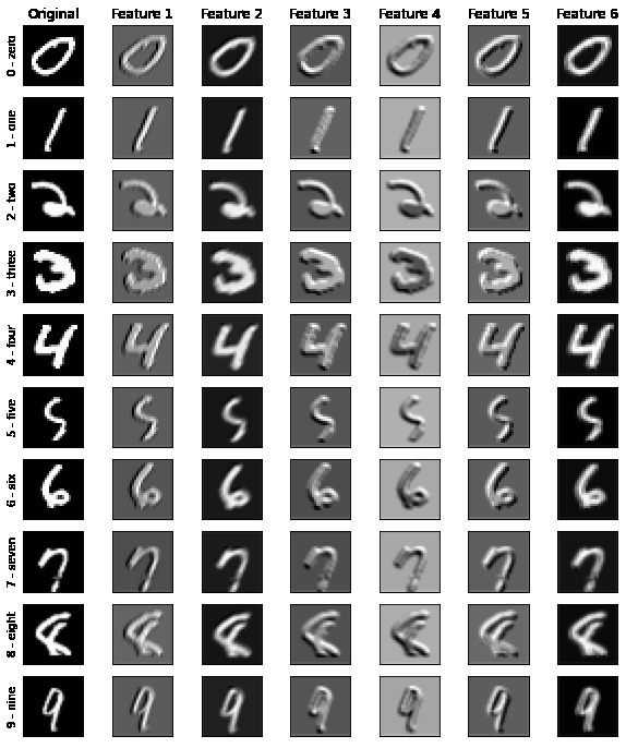
Let’s visualise our Conv layers!
act1 = activations["conv1"]
showActivations(act1, plot_size=(10,12), same_scale=False)
plt.savefig('layer_1_activations.jpg')
act2 = activations["conv2"]
showActivations(act2, plot_size=(20,15), same_scale=False)
plt.savefig('layer_2_activations.jpg')
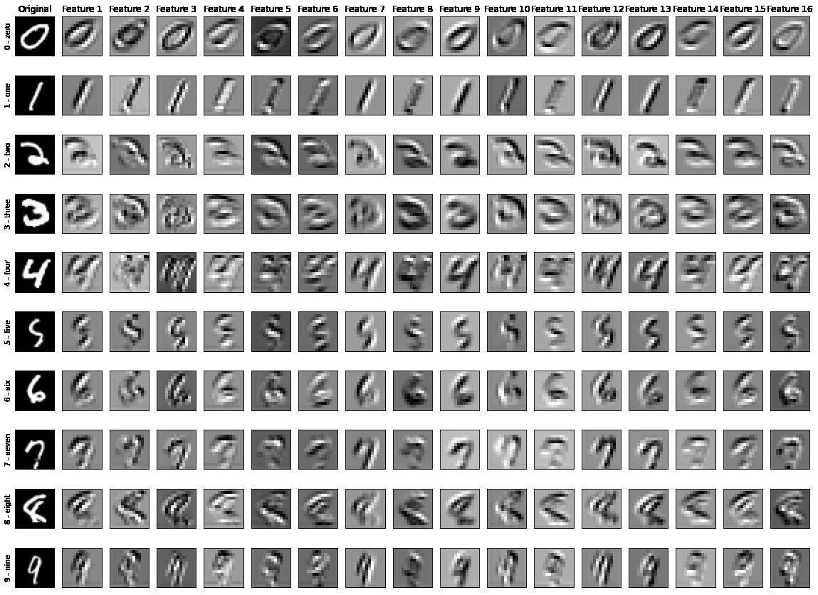
So what can we see - some of our first Conv layer features appear to sharpen the image, accentuating edges. Our second layer features aren’t so clear looking at the activations for a single image, which motivates us to look at the average activations over the entire training set. We sum the activations over the training set, then instead of averaging we scale the colour on our plot to the max/min total activations.
avgAct = torch.zeros((10, 16, 14, 14))
avgOriginals = torch.zeros((10,1,28,28))
# create dataloader of full training set in single batch
train_dataloader_full = torch.utils.data.DataLoader(image_datasets['train'],
                                                    batch_size=len(image_datasets['train']),
                                                    shuffle=True)
imgs, labels = next(iter(train_dataloader_full))
for digit in class_labels:
    idx = (labels==digit).nonzero().squeeze()
    data = imgs[idx]
    avgOriginals[digit] = data.sum(0)
    output = model(data)
    avgAct[digit] = F.relu(activations["conv2"]).sum(0)
data = avgOriginals

showActivations(data, avgAct, plot_size=(20,15), same_scale=True)
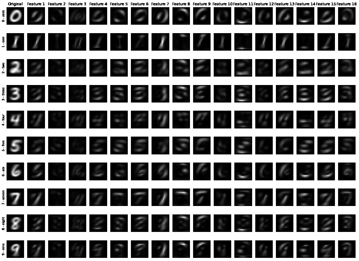
Here we can more clearly interpret what our filters are doing, for example: Feature 7 picks up edges on the right side of the image; Feature 8 the top half; Features 11 and 14 light up to edges curved up at either side like a ‘u’. Its important to note that not all these maps are interpretable to the human eye, but that doesn’t make them redundant as inputs into a classifier.
A final way we can visualise these activations is to look at the total average activation of a feature per digit - to do this we sum our avgAct over the final two indicees, each of size 14, representing the width and height of each image. This gives us an array of size 10 by 16 which we plot as a histogram.
avgAct = []
# select an example from each catagory
# load all training data into one batch
train_dataloader_full = torch.utils.data.DataLoader(image_datasets['train'],
                                                    batch_size=len(image_datasets['train']),
                                                    shuffle=True)

imgs, labels = next(iter(train_dataloader_full))
for digit in class_labels:
    idx = (labels==digit).nonzero().squeeze()
    data = imgs[idx]
    output = model(data)
    avgAct.append(F.relu(activations["conv2"]).sum((2,3)))

bins = np.linspace(0, 40, 100)
fig, axarr = plt.subplots(4, 4, figsize=(17,9))
plt.tight_layout()

for i in range(4):
    for j in range(4):
        axarr[i, j].set_title("Feature "+str(4*i+j+1))
        axarr[i, j].set_yticks([])
        for k in range(len(class_labels)):
            axarr[i, j].hist(avgAct[k][:, 4*i+j], bins, alpha=0.5, label=class_names[k])
plt.legend()
plt.show()
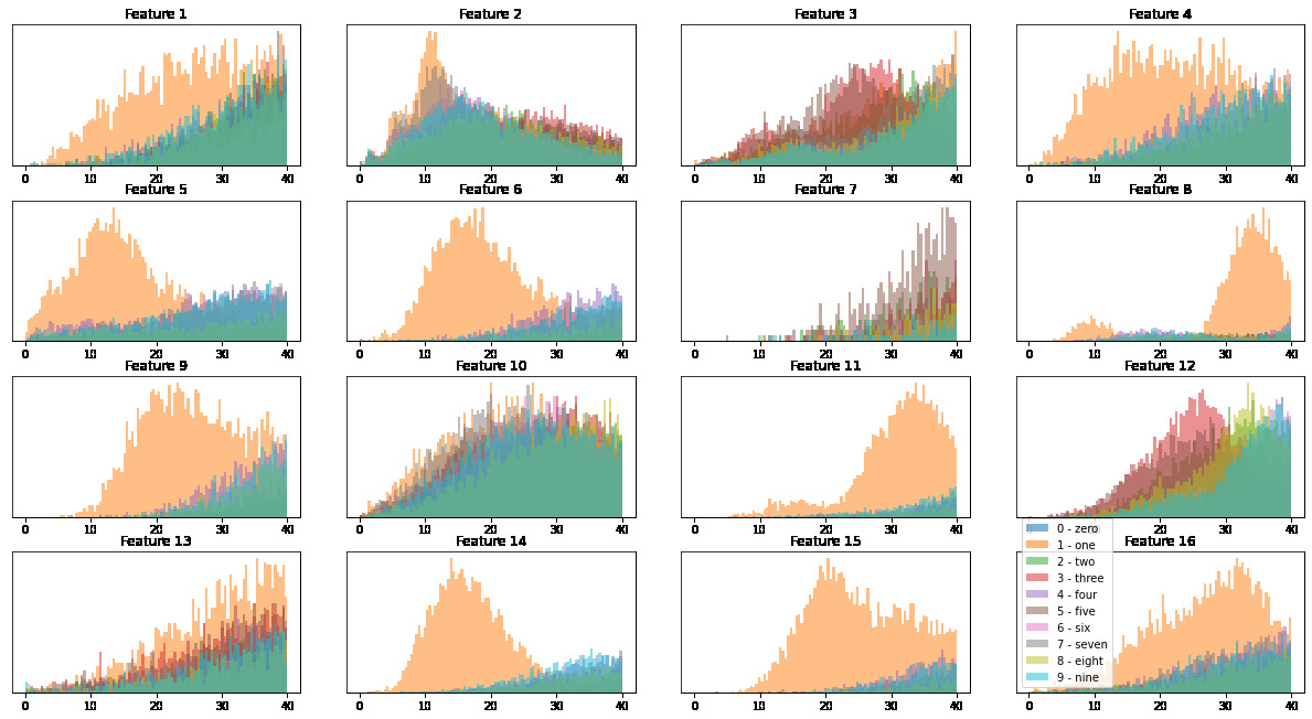
We can see how each class reacts differently to each class, with ‘one - 1’ clearly activiated the most across features. The feature space is able to seperate the dataset well enough that our MLP is able to classify the images to high accuracy.
Conclusion
Interpretability is an increasingly important part of any Machine Learning model, particularly in Deep Learning. Visualising feature maps of a CNN are a step towards understanding why our model classifies the way it does, in just a few extra lines of code. Below are some resources I found interesting.
Further reading
- For an outstanding, detailed and clear introduction to CNNs for Deep Learning, visit the Stanford CS231n notes.
- Distill publish a lot of work on visualisations, a good place to start is this piece on circuits and on interpretability
- Towards Data Science go through a similar visualisation for the massive VGG-net.
For those interested, the Jupyter notebook with code for this post can be found on Github here.